In this module, we will start integrating skills from the previous modules, both about iteration and about data structures, indexing, slicing, etc. We will simulate the temporal dynamics of two populations, one of hosts and one of parasitoids, using a simple time-discrete model.

The Nicholson-Bailey model of host-parasitoid dynamics is a discrete time model where the population size of the host at the next timestep is $H_{t+1} = kH_te^{-aP_t}$, and the population of the parasitoid at the next timestep is $P_{t+1} = cH_t(1-e^{-aP_t})$. In this model, $k$ is the reproductive rate of the host, $c$ is the number of eggs laid in a host, and $a$ is a measure of how actively the parasitoid is looking for its host.

We can easily represent our model as a matrix, with one row for each population, and one column for each timestep:

timeseries = zeros(Float64, 2, 36);

We can also store our parameters in a NamedTuple - this will make it easier to access them in the loop:

parameters = (k = 1.5, c = 1.2, a = 1.02)

(k = 1.5, c = 1.2, a = 1.02)

We need to set our initial populations to something that is not 0! This is very important, as $(0,0)$ is an equilibrium of the model for which neither population grows.

timeseries[1, 1], timeseries[2, 1] = (1.0, 1.0)

(1.0, 1.0)

And now, we can start iterating:

for t in axes(timeseries, 2)
    if t > 1 # We have fixed the initial population
        H, P = timeseries[:, t - 1] # Notice the slice!
        timeseries[1, t] = parameters.k * H * exp(-parameters.a * P)
        timeseries[2, t] = parameters.c * H * (1.0 - exp(-parameters.a * P))
    end
end

We can plot the output of this simulation. This is a lot of Makie code, specifically using the CairoMakie package as we do not need advanced GPU support. This is not really important, but Makie is an excellent plotting package and especially pleasant to work with when using complex layout.

using CairoMakie
CairoMakie.activate!(; px_per_unit = 2) # This ensures high-res figures

The code to generate the figure is as follows:

figure = Figure(; resolution = (600, 600), fontsize = 20, backgroundcolor = :transparent)

The first step is to define an axis, with a scale and labels, and to add a scatterline to it:

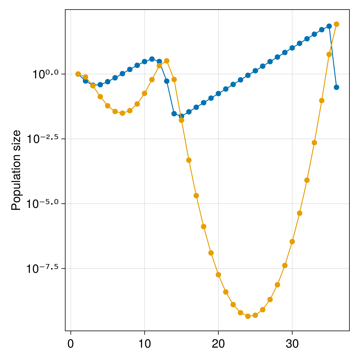
mainplot = Axis(figure[1, 1:2]; ylabel = "Population size", yscale = log10)

scatterlines!(
    mainplot,
    axes(timeseries, 2),
    timeseries[1, :];
    label = "Hosts",
)

scatterlines!(
    mainplot,
    axes(timeseries, 2),
    timeseries[2, :];
    label = "Parasitoids",
)

current_figure()

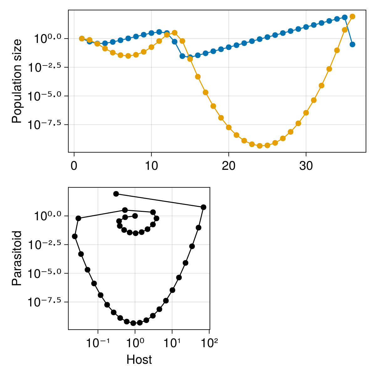
We will add a second axis for the phase plot, and then add the points corresponding to the timeseries:

subplot = Axis(
    figure[2, 1];
    xlabel = "Host",
    ylabel = "Parasitoid",
    xscale = log10,
    yscale = log10,
)

scatterlines!(subplot, timeseries[1, :], timeseries[2, :]; color = :black)

current_figure()

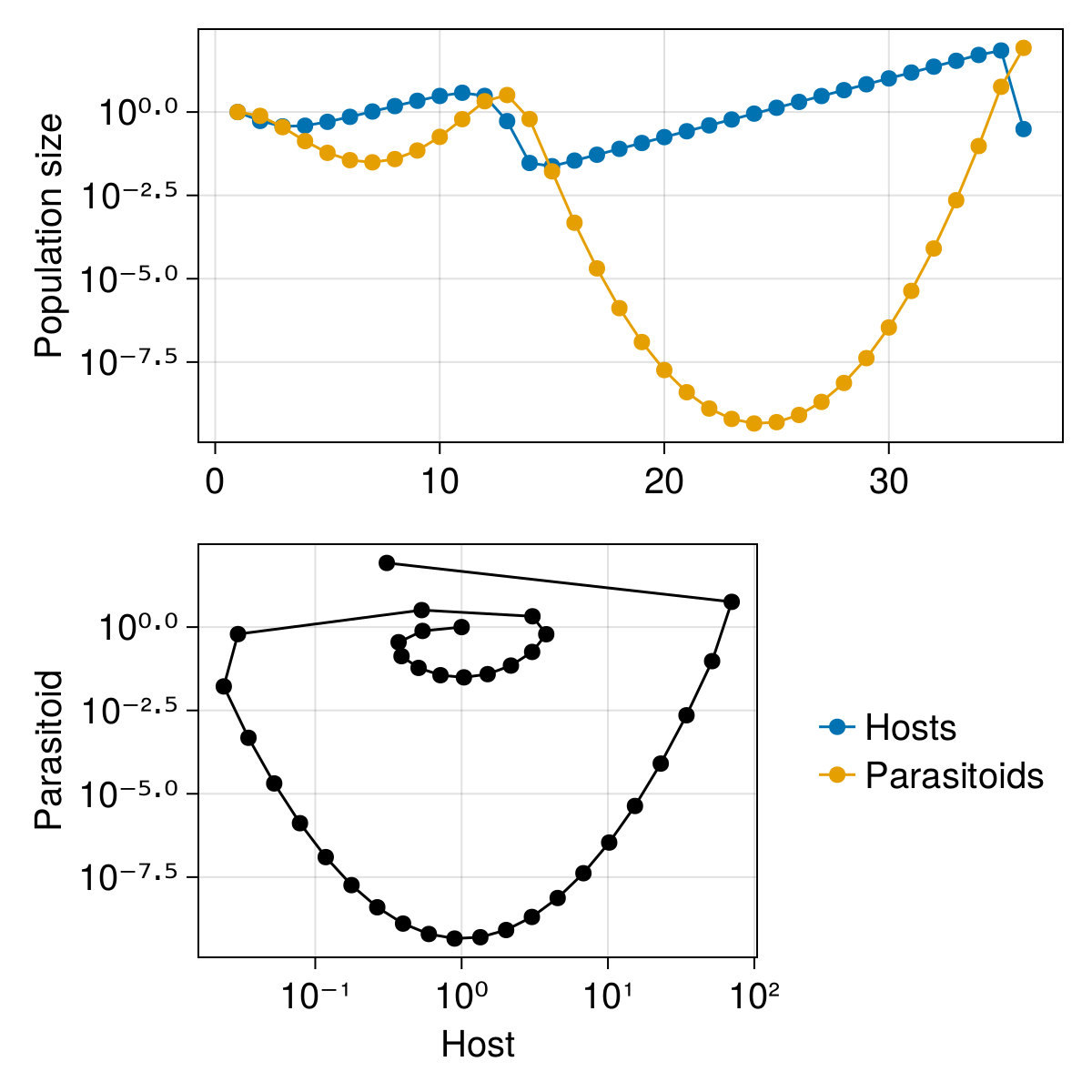
Finally, we can add the legend to the side of the phase plane:

legend = Legend(figure[2, 2], mainplot; framevisible = false)
legend.tellheight = false
legend.tellwidth = true
current_figure()

This wraps the module on iteration. In the next modules, we will go through additional structures to control the flow of our programs.