The travelling salesperson problem · Scientific computing

In this module, we will look at a way to start working on the travelling salesperson problem. This is mostly an excuse to play with simulated annealing, which is a really cool optimisation algorithm.

The travelling salesperson problem is a rather famous problem in optimisation, which is often stated as follows: “given a list of cities represented by their coordinates, what is the shortest possible route that visits all of these cities exactly once, and returns to its origin?”.

using CairoMakie
CairoMakie.activate!(; px_per_unit = 2) # This ensures high-res figures

As this problem involves some stochasticity, we will set a seed for our random number generator, using the Random package from the standard library:

import Random
Random.seed!(12345678)

Random.TaskLocalRNG()

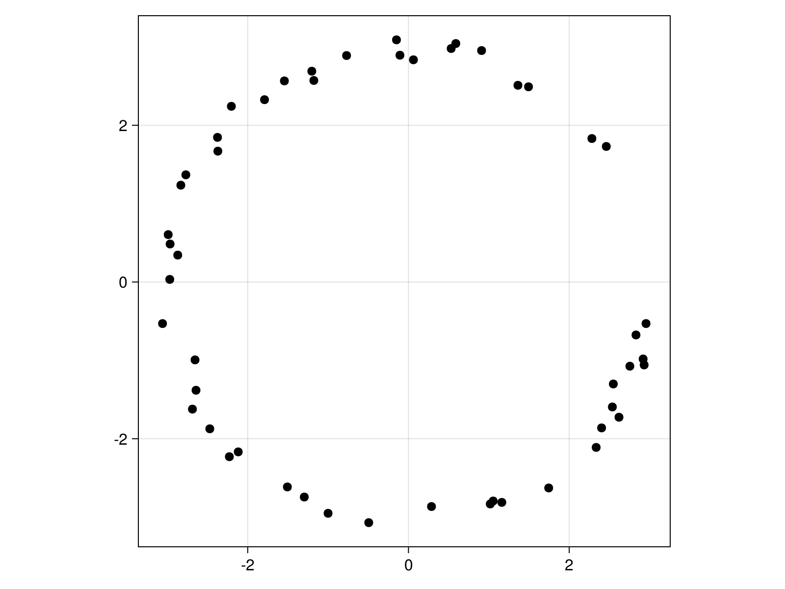
There is a lot of information in this statement, and we will need to translate it into code. But we can work on these elements one at a time. First, there is a list of cities, and these cities are represented by their coordinates. We can set a few limits here: first the world exists in two dimensions; second, there are 50 cities to visit. We will arrange these cities on a circle, with some small perturbations:

angles = rand(50) .* 2π
radii = sqrt.(8.0 .+ rand(length(angles)) .* 2.0)
x = cos.(angles) .* radii
y = sin.(angles) .* radii

cities = permutedims(hcat(x, y))

cities[:, 1:5]

2×5 Matrix{Float64}:
  2.91931   -0.494452  -0.770191   2.4027   -2.68794
 -0.982319  -3.07068    2.88993   -1.86142  -1.62203

We use the square root transform of the radius to have points defined uniformly within a ribbon. This is a small detail, but it’s worth keeping in mind if you want to generate points that are uniformly distributed within a circle.

scatter(
    cities;
    color = :black,
    axis = (; aspect = AxisAspect(1.0)),
    figure = (; backgroundcolor = :transparent),
)

The next information given by the statement of the problem is that we care about the distances between these cities, and so we can pre-calculate these distances, assuming that the Euclidean distance is suitable here.

We need to fill our matrix - this is going to be made easier by the fact that the distance is symmetric, but this is not a requirement here. We will use the foo/foo! design pattern to write two functions to perform this operation.

function distancematrix!(
    D::Matrix{T1},
    cities::Matrix{T2},
) where {T1 <: AbstractFloat, T2 <: AbstractFloat}
    for i in axes(cities, 2)[1:(end - 1)], j in axes(cities, 2)[(i + 1):end]
        D[i, j] = D[j, i] = sqrt(sum((cities[:, i] .- cities[:, j]) .^ 2.0))
    end
    return D
end

distancematrix! (generic function with 1 method)

We are using different floating point precisions here because the distance matrix might be large, and because we don’t really care about getting a lot of precision. By default, we will use Float16.

function distancematrix(cities::Matrix{T}; dtype::Type = Float16) where {T <: Number}
    D = zeros(dtype, size(cities, 2), size(cities, 2))
    return distancematrix!(D, cities)
end

distancematrix (generic function with 1 method)

With these two functions, we can generate our distance matrix:

D = distancematrix(cities; dtype = Float16);

The third element of the problem is that we have a “route”, which is the order in which we visit cities. Each city is visited only once (so we know how many stops there are), and the salesperson returns to the origin city.

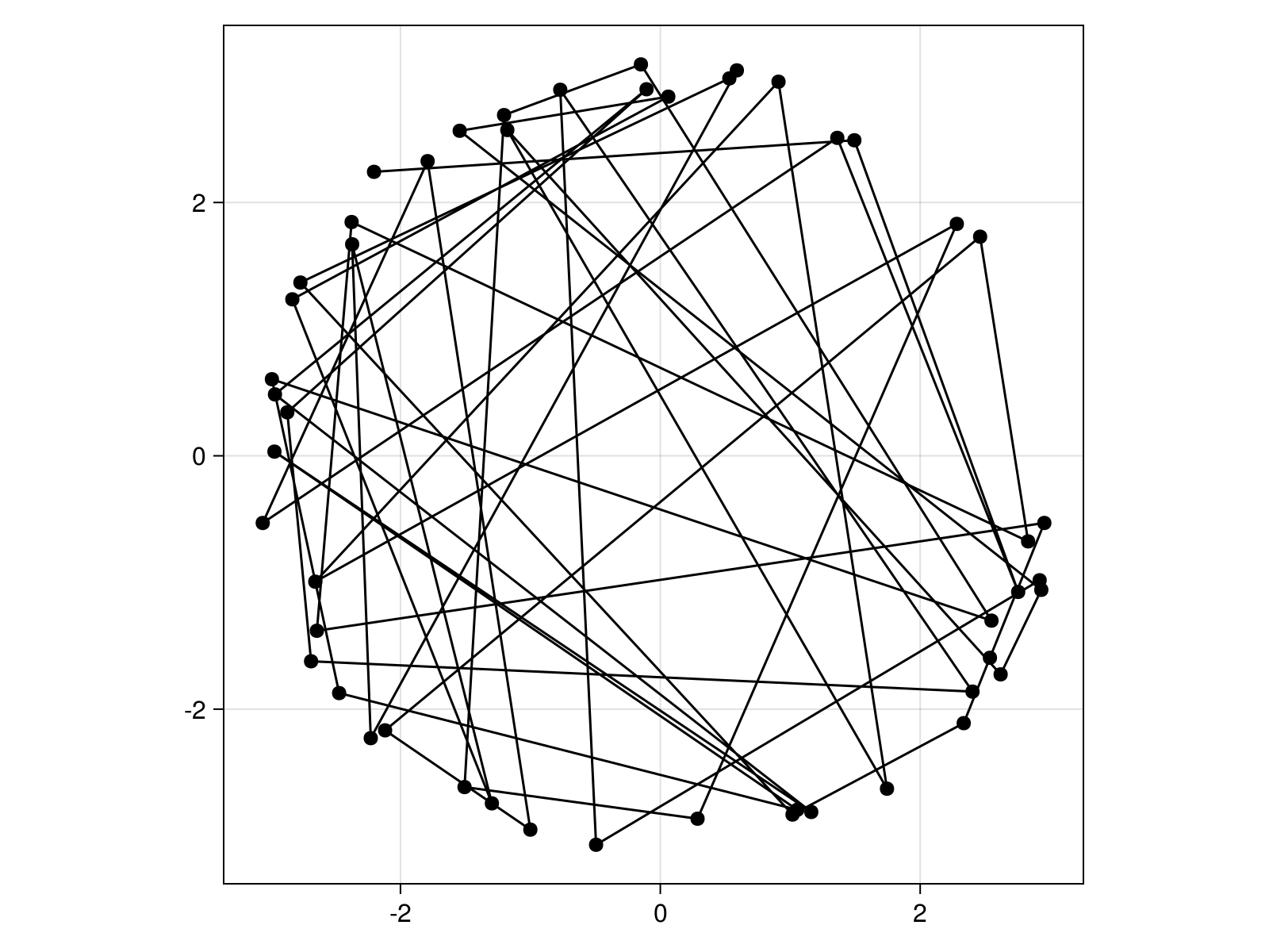
We do not really care about which city is the origin city, since by the end, we will have a loop. We can simply pick whichever arbitrary city we want as the point of origin after the fact.

The easiest way to represent a route is therefore to have a series of indices, representing the order in which we visit the cities. In the absence of a know initial solution, we will simply visit the cities in order:

route = collect(axes(cities, 2));

We can plot this route to see what it would look like:

scatter(
    cities;
    color = :black,
    axis = (; aspect = AxisAspect(1.0)),
    figure = (; backgroundcolor = :transparent),
)
lines!(cities[:, route]; color = :black)
current_figure()

What is the total travel distance of this route? In order to know this, we only need to read the pairwise distances between adjacent cities in the route, and add the return step at the end. This is feasible with a list comprehension, as we need to read the distance between step $i$ and step $i-1$ of the route, which are mapped to two different cities:

function routedistance(route, D)
    pairwise_distances = [D[route[i - 1], route[i]] for i in axes(route, 1)[2:end]]
    return_home = D[route[end], route[begin]]
    return sum(pairwise_distances) + return_home
end

routedistance (generic function with 1 method)

We know that our distance matrix is not going to change, so in the spirit of being very lazy, we can add a method to routedistance that returns a function based on distance matrix:

function routedistance(D)
    return (route) -> routedistance(route, D)
end

routedistance (generic function with 2 methods)

We can use this function to write our distance calculator:

RD = routedistance(D)

#4 (generic function with 1 method)

With this function, we can calculate our current best distance ($d_0$):

δ₀ = RD(route)

Float16(202.6)

Problem solved! Now what we need to do is find a way to decrease this distance, which would represent a shortest path. We could brute-force our way through the solution, but this would take a lot of time. Instead, we are going to rely on simulated annealing to optimize the problem for us, in a way that is going to be able to jump over local minima.

In simulated annealing, we have an energy budget, which is exhausted in a time-dependent way, which can be exponential, inverse-log, or geometric (the function we will implement here). The energy budget serves to calculate the probability of accepting a bad move, i.e. a move that would make the route longer.

function energy(T₀, λ, t)
    return T₀ * (λ^t)
end

energy (generic function with 1 method)

Accepting a bad move is based on a probability, which is given by the exponential of minus the cost of the move divided by the energy. The cost of the move, in turn, is defined as the differentce between the route length and the best route length so far:

function move_probability(δᵢ, δ₀, ε)
    return exp(-(δᵢ - δ₀) / ε)
end

move_probability (generic function with 1 method)

The best distance, initially, is given by δ₀. We need to define what a move is. There are a few different ways, but the simplest one is probably to switch the order in which we visit two cities. We can pick to positions in the route with:

switch = rand(eachindex(route), 2)

2-element Vector{Int64}:
  4
 44

This corresponds to two cities:

route[switch]

2-element Vector{Int64}:
  4
 44

We can now flip them by changing the route in place:

route[switch] = route[reverse(switch)]

2-element Vector{Int64}:
 44
  4

And we now have all of the ingredients to build our simulated annealing optimisation of the travelling salesperson problem! All we need to do is run it a long enough time. The secret in simulated annealing is to use a long run time with a very gradual cooling schedule.

best_distance = zeros(Float64, 200_000)
best_distance[1] = δ₀

Float16(202.6)

We now have everything we need to run the algorithm. If a move is good, we will always accept it, and if it is bad, we will accept it with a probability dependent on the current energy of the system. We need to decide on a value for T₀ and λ, which require some manual tweaking. As a good heuristic, starting with an initial temperature equal to twice the best solution often “just works”, and a value of the decay parameter very close to unity ensures that the cooling is very gradual.

T₀, λ = 2δ₀, 0.9999

(Float16(405.2), 0.9999)

We can now run everything. This problem is very simple, so this will only take a few seconds. We will use @elapsed in front of the loop, to se how many seconds it actually took:

@elapsed for i in axes(best_distance, 1)[2:end]
    local switch
    switch = rand(eachindex(route), 2)
    route[switch] = route[reverse(switch)]
    δᵢ = RD(route)
    if δᵢ < best_distance[i - 1]
        best_distance[i] = δᵢ
    else
        if rand() <= move_probability(δᵢ, best_distance[i - 1], energy(T₀, λ, i))
            best_distance[i] = δᵢ
        else
            route[switch] = route[reverse(switch)]
            best_distance[i] = best_distance[i - 1]
        end
    end
end

0.418439641

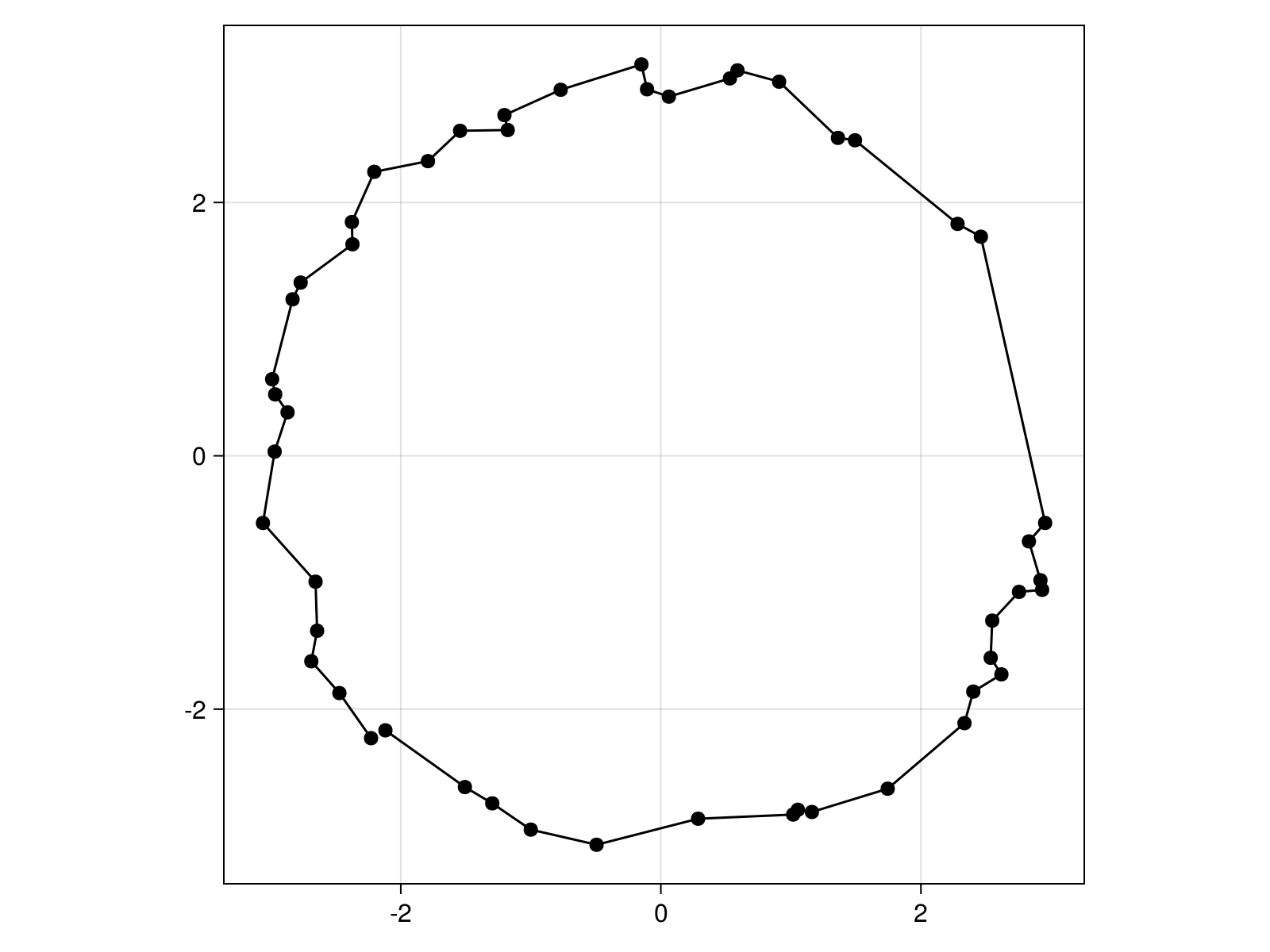
After all the iterations are done, we can have a look at the new solution:

scatter(
    cities;
    color = :black,
    axis = (; aspect = AxisAspect(1.0)),
    figure = (; backgroundcolor = :transparent),
)
lines!(cities[:, route]; color = :black)
current_figure()

We can also check that the solution has been getting better over time, by looking at the distance:

lines(
    log.(best_distance);
    axis = (; xlabel = "Step", ylabel = "Route distance (log)"),
    figure = (; backgroundcolor = :transparent),
)

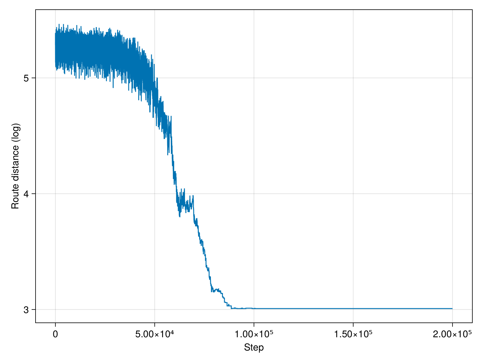
This works rather well!

If we’re being fully honest? We tried different seeds for the random number generator until finding one that gave the “perfect” result. Sorry.

An interesting observation is that the shortest distance had not changed for a large number of iterations. This is because the energy in the system was very close to 0, and so even a barely bad move had no chance of being accepted. A possible refinement of this algorithm would be to keep track of the number of steps since there was last an improvement, and fix a point at which we stop.