In this module, we will have a look at indexing in order to simulate the behavior of a forest when trees can catch on fire, be planted, and regrow. This is a common example in complex system studies, and produces very visually pleasing structures in space! As a treat, we will spend a little more time learning about how Makie works.

This applications is inspired by the chapter on forest fire dynamics in Paul Charbonneau’s book on natural complexity, which is extremely well written and illustrated, and full of applications (with Python) code to explore the behavior of complex systems.

We will rely on CairoMakie for plotting, and nothing else!

using CairoMakie
CairoMakie.activate!(; px_per_unit = 2)

The first decision we need to make it to set a grid for the size of our forest. Large grids take more time to simulate, and the number of cells is the square of the grid dimension. A large grid will let us see the grey corresponding to patches of re-growing forest, but a small grid will run much faster.

grid_size = (550, 550)

(550, 550)

We will use the following convention: an empty cell is 0, a burning cell is 1, and a planted cell is 2. The reason we are using numbers here is that they take less memory footprint than strings or symbols would, and that’s about it. There are many other ways to solve this problem, including defining an enumerated type, or a type for each state, but using a basic type will also have the benefit of mapping directly into colormaps for visualization, and to let us use the iszero and isone to pick the empty and burning pixels.

forest = zeros(Int64, grid_size .+ 2);
forestchange = zeros(Int64, grid_size .+ 2);

You might notice that we are cheating a little bit by assigning a larger grid than we decided. There is a simple reason for this: we will spend time looking at the neighborhood of pixels, and it is faster to pad the grid with empty states than it is to filter the neighborhood to ensure that all of the positions are in the grid. Thankfully, we know how to use slices like [(begin+1):(end-1)] to handle this!

The next step is to decide on two probabilities: the probability of a tree appearing in an empty cell (assume that birds are dispersing the seeds, and that trees appear fully mature), $p$; and the probability that a fire will start in a pixel occupied by a tree, $f$ (this is usually assumed to be the effect of lightning, for example).

p = 1e-2
S = 130
f = p * (1 / S)

7.692307692307693e-5

One of the rules of the model is that a tree on fire will propagate the “burning” state to its neighbors. In order to do this, we can define a “stencil”, or a collection of relative positions one-next to the focal cell:

CartesianIndices((-1:1, -1:1))

CartesianIndices((-1:1, -1:1))

This is nothing more than a square matrix wearing a trench coat:

collect(CartesianIndices((-1:1, -1:1)))

3×3 Matrix{CartesianIndex{2}}:
 CartesianIndex(-1, -1)  CartesianIndex(-1, 0)  CartesianIndex(-1, 1)
 CartesianIndex(0, -1)   CartesianIndex(0, 0)   CartesianIndex(0, 1)
 CartesianIndex(1, -1)   CartesianIndex(1, 0)   CartesianIndex(1, 1)

The reason we are not assigning this to a variable is because we will pass it as a keyword argument to our simulation function later on. In order to have a starting state, we will seed the landscape with a few trees:

locations_to_plant = filter(i -> rand() <= p, eachindex(forest[2:(end - 1), 2:(end - 1)]))
forest[locations_to_plant] .= 2;

We will soon want to gaze upon the greatness that is our simulation, so it makes sense to create a color gradient to pass to the heatmap function – we will use white for empty cells, orange for active fires, and green for trees. We also specify that this gradient has three categorical endpoints, so that our three categories will map to their colors.

fire_state_palette = cgrad([:white, :orange, :green], 3; categorical = true)

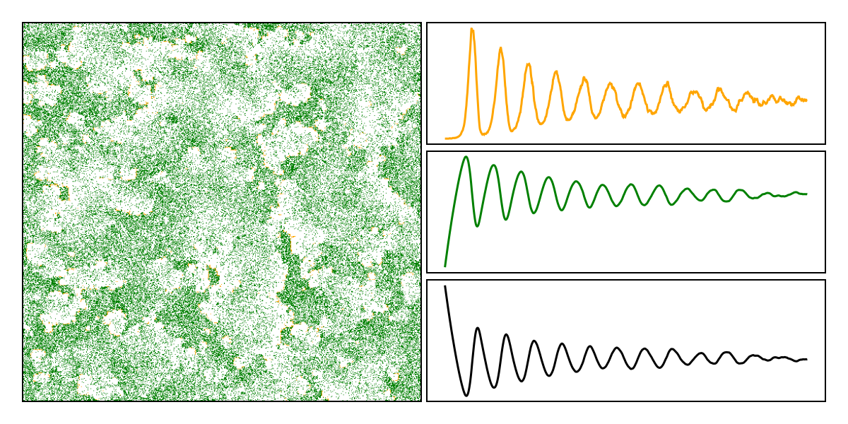
In order to keep track of everything, we will setup a figure with four panels. The heatmap representing the state of our forest, and then the time series for the number of burning, planted, and empty pixels on the right.

figure = Figure(; resolution = (600, 300), fontsize = 20, backgroundcolor = :transparent)
forest_plot = Axis(figure[1:3, 1])
B_plot = Axis(figure[1, 2])
P_plot = Axis(figure[2, 2])
V_plot = Axis(figure[3, 2])
current_figure()

Because the numbers do not really matter, we can hide all of the decorations, and also tighten the layout a little bit to avoid the big gap between panels:

hidedecorations!(forest_plot)
hidedecorations!(B_plot)
hidedecorations!(P_plot)
hidedecorations!(V_plot)
rowgap!(figure.layout, 5)
colgap!(figure.layout, 5)
current_figure()

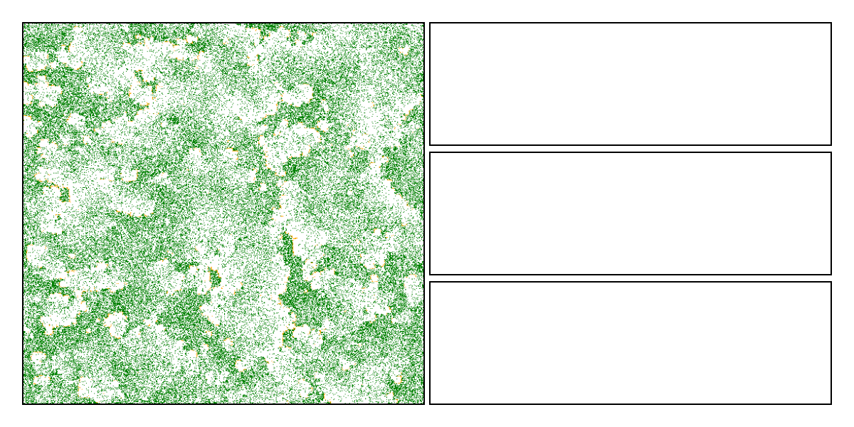
And we can start by showing the initial state of our forest, which is mostly empty with a small number of spatially unstructured trees:

heatmap!(forest_plot, forest; colormap = fire_state_palette)
current_figure()

Because this is an iterative model, i.e. we will run it a lot of times to look at its behavior, we need to define our epochs:

epochs = 1:1000

1:1000

To keep track of the state of the model, we will pre-allocate a number of empty arrays:

V = zeros(Int64, length(epochs));
P = zeros(Int64, length(epochs));
B = zeros(Int64, length(epochs));

We are now ready to start implementing the model. It is a simple model (as complex systems often are), with four rules, that are executed simultaneously. The first rule of the forest fire model is that trees appear in empty pixels at a set probability $p$. It may be tempting to iterate now, but let’s see what the other rules are first.

The second rule of the model is that trees catch fire at random when struck by lightning (with probability $f$). The third rule is that a burning tree immediately dies oof and becomes an empty pixel. The final rule is that any tree next to a burning tree will catch on fire.

Well, it definitely does not makes sense to iterate over the entire forest for each of these rules, so we will write a longer function that only iterates once. But in the spirit of writing small functions, we will first implement the rules as function of their own.

The first rule is simple: if the empty cell gets a tree, we change its value in the matrix of change:

function _manage_empty_cells!(change, state, position, p_tree)
    if rand() <= p_tree
        setindex!(change, 2, position)
    else
        setindex!(change, 0, position)
    end
    return nothing
end

_manage_empty_cells! (generic function with 1 method)

The second rule is very similar:

function _manage_planted_cells!(change, state, position, p_fire)
    if rand() <= p_fire
        setindex!(change, 1, position)
    end
    return nothing
end

_manage_planted_cells! (generic function with 1 method)

The third rule is a little more complex, as we will need to account for the dispersal kernel, which we will pass as a final argument:

function _manage_burning_cells!(change, state, position, kernel)
    for surrounding in kernel
        if state[position + surrounding] == 2
            setindex!(change, 1, position + surrounding)
        end
    end
    setindex!(change, 0, position)
    return nothing
end

_manage_burning_cells! (generic function with 1 method)

We can now wrap everything in a function called fire!:

function fire!(change, state, p_tree, p_fire; kernel = CartesianIndices((-1:1, -1:1)))
    used_indices = CartesianIndices(forest)[(begin + 1):(end - 1), (begin + 1):(end - 1)]
    for pixel_position in used_indices
        if state[pixel_position] == 0
            _manage_empty_cells!(change, state, pixel_position, p_tree)
        elseif state[pixel_position] == 2
            _manage_planted_cells!(change, state, pixel_position, p_fire)
        elseif state[pixel_position] == 1
            _manage_burning_cells!(change, state, pixel_position, kernel)
        end
    end
    for pixel_position in used_indices
        state[pixel_position] = change[pixel_position]
        change[pixel_position] = state[pixel_position]
    end
    return (count(iszero, state), count(isone, state), count(isequal(2), state))
end

fire! (generic function with 1 method)

We can test that this function works by counting the number of trees in the new state matrix before:

count(isequal(2), forest)

2947

And after:

fire!(forestchange, forest, p, f)

(301597, 1, 3106)

Equipped with this function, it is very simple to repeat the cycle until all of the epochs have been done:

for epoch in epochs
    V[epoch], B[epoch], P[epoch] = fire!(forestchange, forest, p, f)
end

This simulation may take a little time, as we could optimize a number of things. Notably, this problem is very easy to distribute across multiple threads, which could give a solid speed-up. But at the end, we can overwrite the panel with the state of the forest:

heatmap!(forest_plot, forest; colormap = fire_state_palette)
current_figure()

And then we can add the dynamics of the different categories of pixels, to see the oscillations hapenning:

lines!(P_plot, P; color = :green)
lines!(B_plot, B; color = :orange)
lines!(V_plot, V; color = :black)
current_figure()