In this module, we will use the gradient descent algorithm to perform a linear regression, to estimate the brain mass of an animal if we know its body mass. This will draw on concepts from a number of previous modules, while also presenting an example of how core programming skills can be applied for research.

using Distributions
using CairoMakie
CairoMakie.activate!(; px_per_unit = 2) # This ensures high-res figures

Here is a broad overview of the task we want to accomplish. The AnimalTraits database provides curated information about metabolic rates of several species of animals. There is a linear relationship between the log of body mass and the log of brain size (both expressed in kg). In this module, we will estimate the parameters of this relationship using linear regression for birds.

We will first download, then load, the data – we use the CSV.File approach here, which is great for structured data, and accepts a lot of different options to only read the required columns (see ?CSV.File for more!). CSV has plenty of additional features, and works really well with e.g. DataFrames.

We will limit the output to the first three rows:

import CSV
data_url = "https://zenodo.org/record/6468938/files/observations.csv?download=1"
data_file = download(data_url)
traits = CSV.File(data_file; delim = ",", select = ["class", "body mass", "brain size"])
traits[1:3]

3-element Vector{CSV.Row}:
 CSV.Row:
 :class                 "Amphibia"
 Symbol("body mass")   0.01315
 Symbol("brain size")  4.225844e-5
 CSV.Row:
 :class                 "Amphibia"
 Symbol("body mass")   0.0001
 Symbol("brain size")  2.25848e-6
 CSV.Row:
 :class                 "Amphibia"
 Symbol("body mass")   0.0003
 Symbol("brain size")  4.43408e-6

Because some species have missing values, we can use a combination of filter and any to remove them:

traits = filter(v -> all(.!ismissing.(v)), traits)
traits = filter(v -> v.class == "Aves", traits)
traits[1:3]

3-element Vector{CSV.Row}:
 CSV.Row:
 :class                  "Aves"
 Symbol("body mass")   43.85
 Symbol("brain size")   0.0376586
 CSV.Row:
 :class                  "Aves"
 Symbol("body mass")   36.5
 Symbol("brain size")   0.02991968
 CSV.Row:
 :class                 "Aves"
 Symbol("body mass")   2.3
 Symbol("brain size")  0.00588448

We will now extract our vectors $x$ (body mass, the predictor) and $y$ (body mass, the response), and pass them through the log10 function to have a linear relationship:

X = log10.([trait[Symbol("body mass")] for trait in traits]);
Y = log10.([trait[Symbol("brain size")] for trait in traits]);

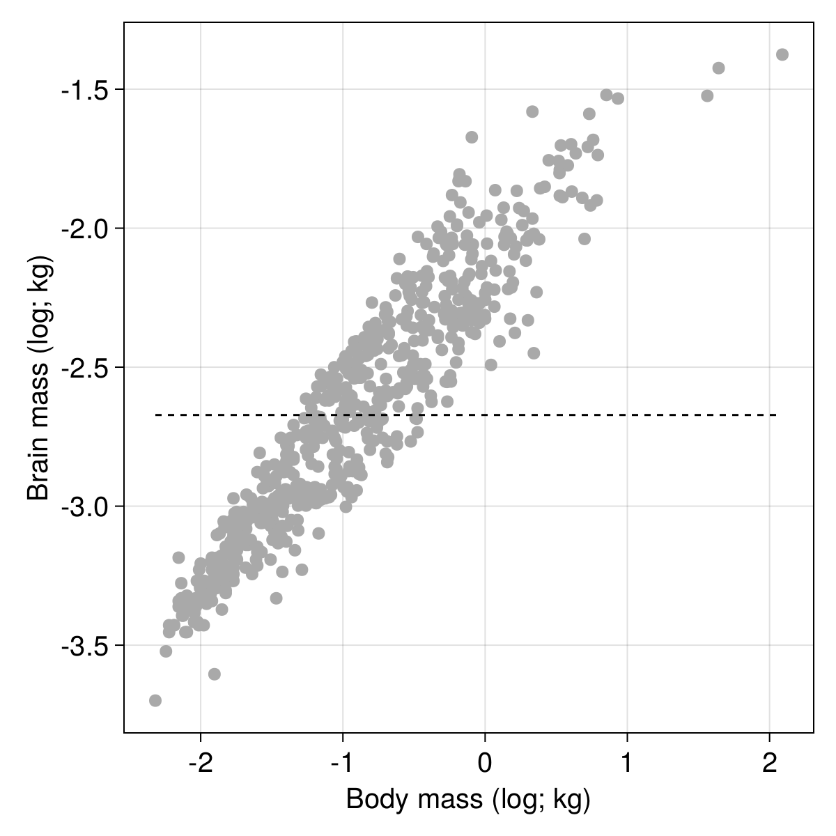
It is always a good idea to look at the data before attempting any modelling, so we can use the CairoMakie package to do so:

figure = Figure(; resolution = (600, 600), fontsize = 20, backgroundcolor = :transparent)
scplot = Axis(figure[1, 1]; xlabel = "Body mass (log; kg)", ylabel = "Brain mass (log; kg)")
scatter!(scplot, X, Y; color = :darkgrey)
current_figure()

After checking that the relationship between $Y$ and $X$ looks suitably linear, we can start thinking about the optimization algorithm. Optimization requires a target, otherwise known as a loss function. We will use the mean squared error estimator, which as its name suggests, compare the actual values to the predictions, and returns the sum of their differences squared, divided by the number of elements (to make the score dimensionless with regards to sample size).

ℒ(Y, Ŷ) = sum((Y .- Ŷ) .^ 2.0) / length(Y)

ℒ (generic function with 1 method)

We can measure the loss that we would get based on no slope and an intercept equal to the average of $y$:

using Statistics
m₀, b₀ = 0.0, mean(Y)
Ŷ₀ = m₀ .* X .+ b₀
ℒ(Y, Ŷ₀)

0.20123658885902382

It’s not very good! We can get visual confirmation of the poor fit by adding a line to our plot:

lines!(
    scplot,
    [minimum(X), maximum(X)],
    (x) -> m₀ .* x .+ b₀;
    color = :black,
    linestyle = :dash,
)
current_figure()

How do we fix this? The gradient descent algorithm works by mapping the loss value $L$ to the parameters values. Specifically, the gradient is given by

$$ \nabla f = \begin{bmatrix} \frac{\partial L}{\partial m} && \frac{\partial L}{\partial b} \end{bmatrix}^\intercal $$

The value of $\partial L/\partial m$ is the partial derivative of the loss function with regards to $m$, and can be calculated from the definition of the loss function. In Julia, there are a number of autodiff packages like Zygote who make this task a lot easier, but for the purpose of this example, it is a good idea to see what we can build out of the base language.

After some calculations, we can get the two components of the gradient. We will express them as functions:

∂m(X, Y, Ŷ) = -(2 / length(X)) * sum(X .* (Y .- Ŷ));
∂c(X, Y, Ŷ) = -(2 / length(X)) * sum(Y .- Ŷ);

We can finally wrap these two function within a single function expressing the gradient $\nabla f$:

∇f(X, Y, Ŷ) = [∂m(X, Y, Ŷ), ∂c(X, Y, Ŷ)]

∇f (generic function with 1 method)

In gradient descent, the update scheme for the parameters is very simple; at each iteration, we transform $m$ and $b$ by substracting the values in the gradient. In other words, $\mathbf{p} = \mathbf{p} - \nabla f$, where $\mathbf{p}$ is a column vector storing the parameters.

What is the gradient like at our initial (very bad estimate)? We can call the ∇f function to get the answer:

∇f(X, Y, Ŷ₀)

2-element Vector{Float64}:
 -0.6265421588393548
 -1.7985266595487714e-15

These look like very large values. There are two reasons for this. The first is that our initial guess is, as we have seen from the figure, very bad. Therefore, we expect to move quite far away from the parameter values. The second reason (far more important here) is that we are being a little over-eager in our learning. The risk with learning too much is that we can move so far away that we will miss the correct value, by jumping straight over it.

In order to solve this problem, we will add a learning rate $\eta$, which is a small value (much smaller than 1) by which we will multiply the gradient, so that our update scheme becomes $\mathbf{p} = \mathbf{p} - \eta\times \nabla f$:

η = 1e-3;

We can now check that our move is much smaller in magnitude:

η .* ∇f(X, Y, Ŷ₀)

2-element Vector{Float64}:
 -0.0006265421588393549
 -1.7985266595487716e-18

Excellent! With these elements, we are ready to start solving our problem. We can generate an initial solution at random:

𝐩 = rand(2)

2-element Vector{Float64}:
 0.8123352258345882
 0.2415581580177376

And now, we very simply iterate over a set number of epochs (both the number of epochs and the learning rate are hyperparameters of the model), updating the values of $\mathbf{p}$ as we go along:

epochs = 10_000
for i in 1:epochs
    𝐩 .-= η .* ∇f(X, Y, 𝐩[1] .* X .+ 𝐩[2])
end

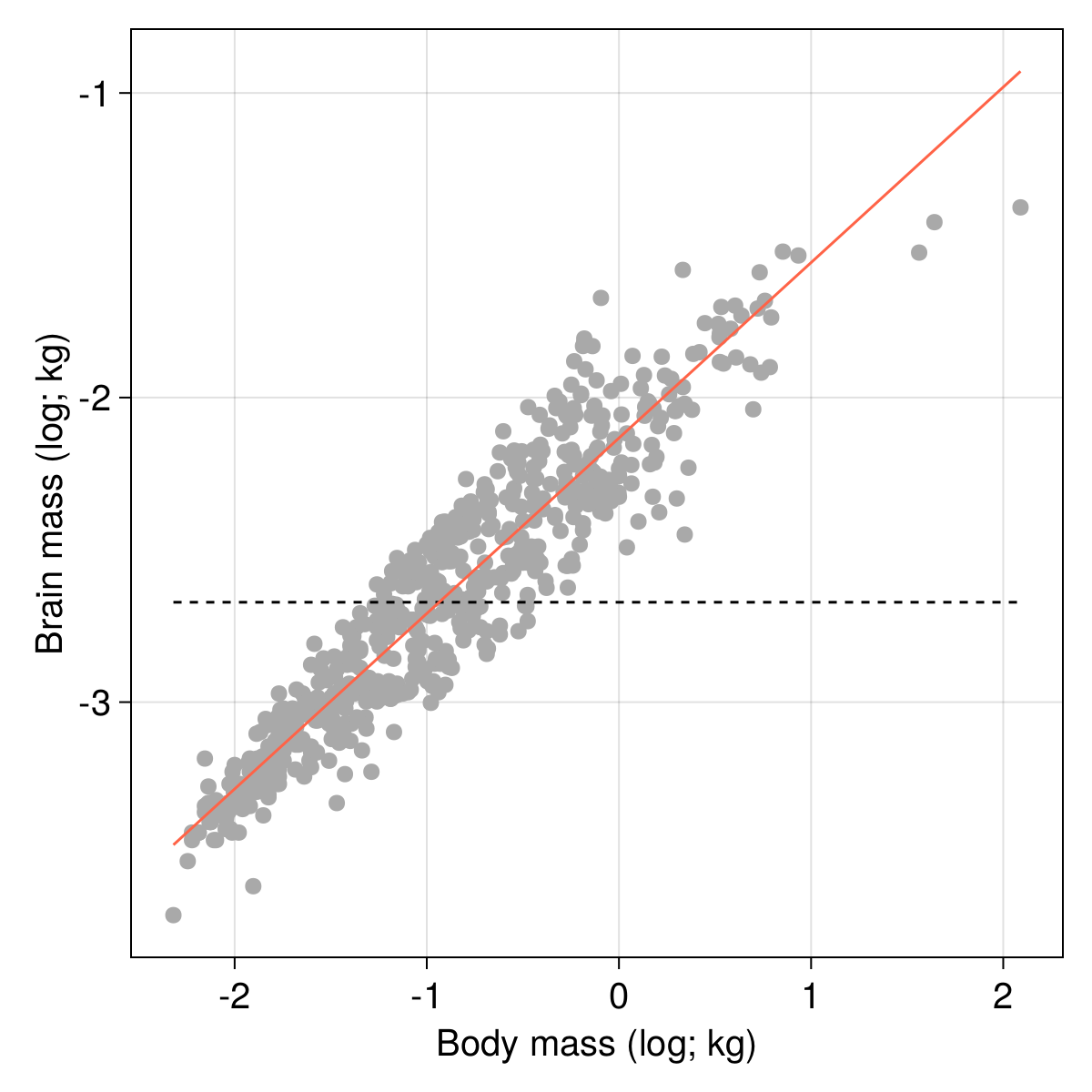
After the training epochs are done, we can get a look at the result (note that we use a ternary expression to decide how to report the sign of the elevation). We mostly care about the value of the loss function, and the value of the parameters:

"""
Best model: ŷ ≈ $(round(𝐩[1]; digits=2))x $(𝐩[2]<0 ? "" : "+") $(round(𝐩[2]; digits=2))
Loss: ℒ ≈ $(round(ℒ(𝐩[1] .* X .+ 𝐩[2], Y); digits=4))
""" |> println

Best model: ŷ ≈ 0.58x  -2.13
Loss: ℒ ≈ 0.0232

As always, visualisation provides a good sanity check of these results, and our line should now be much closer to the cloud of points:

lines!(
    scplot,
    [minimum(X), maximum(X)],
    (x) -> 𝐩[1] .* x .+ 𝐩[2];
    color = :tomato,
)
current_figure()

One noteworthy thing about this example is that building our own (admittedly not very general, and not very efficient) gradient descent optimizer was possible in a very small number of lines of code, and using only functions from Julia’s standard library. There are a lot of packages dedicated to performing this task extremely efficiently; but this example shows how we can easily get to a working solution, which is interesting both for experimenting with new approaches, and for learning new skills.